©2026_NKTg = f(x,v,m)

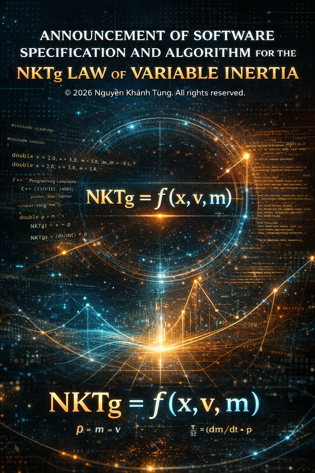
ANNOUNCEMENT OF SOFTWARE SPECIFICATION AND ALGORITHM FOR THE NKTg LAW OF VARIABLE INERTIA

ANNONCE DU DOSSIER DESCRIPTIF DU LOGICIEL ET DE L’ALGORITHME DE LA LOI NKTg SUR L’INERTIE VARIABLE

CÔNG BỐ HỒ SƠ MÔ TẢ PHẦN MỀM VÀ GIẢI THUẬT ĐỊNH LUẬT NKTg VỀ QUÁN TÍNH BIẾN THIÊN

关于 NKTg 变惯性定律的软件规格与算法公告

BEKANNTMACHUNG DER SPEZIFIKATIONEN FÜR SOFTWARE UND ALGORITHMEN DES NKTg-GESETZES ÜBER VARIABLE TRÄGHEIT

NKTg 変位慣性法則に関するソフトウェアおよびアルゴリズム仕様公表

ANUNCIO DE ESPECIFICACIONES DE SOFTWARE Y ALGORITMOS DE LA LEY NKTg DE INERCIA VARIABLE

ПУБЛИКАЦИЯ СПЕЦИФИКАЦИЙ ПРОГРАММНОГО ОБЕСПЕЧЕНИЯ И АЛГОРИТМОВ ЗАКОНА NKTg О ПЕРЕМЕННОЙ ИНЕРЦИИ

1. English (English)

ANNOUNCEMENT OF SOFTWARE SPECIFICATION AND ALGORITHM FOR THE NKTg LAW OF VARIABLE INERTIA

© 2026 Nguyễn Khánh Tùng. All rights reserved.

I. GENERAL INFORMATION

• Software Name:

NKTg Variable Inertia Computing System (NKTg Dynamics Calculator).

• Author:

Nguyễn Khánh Tùng

• Programming Languages:

C++ (ISO/IEC 14882) and Assembly (x64).

II. THEORETICAL BASIS: NKTg LAW OF VARIABLE INERTIA

The software is implemented based on the principles of the NKTg Law:

• Fundamental Relationship:

Movement tendency depends on position (x), velocity (v), and mass (m). Formula: NKTg = f(x, v, m).

• Core Product Quantities:
  • Momentum (p): p = m * v
  • NKTg_1 Quantity: Product of position and momentum (NKTg_1 = x * p).
  • NKTg_2 Quantity: Product of the mass variation rate and momentum (NKTg_2 = (dm/dt) * p).
• Unit of Measurement:

NKTm (Unit of variable inertia).

III. DETAILED ALGORITHM DESCRIPTION

1. Data Processing Workflow

The algorithm performs movement tendency analysis through logical steps:

• Step 1:

Receive input parameters: position (x), velocity (v), mass (m), and mass change rate (dm/dt).

• Step 2:

Calculate linear momentum p = m * v.

• Step 3:

Calculate variable inertia values NKTg_1 and NKTg_2.

• Step 4:

Classify the tendency (Tendency) based on the sign of the value:

• NKTg_1 > 0: Moving away from stable state.
• NKTg_1 < 0: Moving toward stable state.
• NKTg_2 > 0: Mass variation supports movement.
• NKTg_2 < 0: Mass variation resists movement.

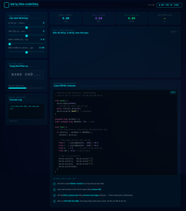
IV. EXECUTION SOURCE CODE (SOURCE CODE)

1. High-Level Source Code (C++)

C++

#include <cstdio>

/**

 * Computational library for Variable Inertia according to NKTg Law

 * All copyrights reserved regarding calculation logic and tendency definitions.

 */

int main() {

   // 1. Declare parameters: x (position), v (velocity), m (mass), dm_dt (mass variation rate m)

   double x = 2.0, v = 3.0, m = 5.0, dm_dt = -0.5;

   // 2. Perform calculation according to NKTg Law

   double p = m * v;        // p = m * v

   double n1 = x * p;       // NKTg1 = x * p

   double n2 = dm_dt * p;   // NKTg2 = (dm/dt) * p

   // 3. Output results in Record format

   printf(“{ p = %.1f\n  nktg1 = %.1f\n  nktg2 = %.1f\n”, p, n1, n2);

   // Movement Tendency Classification (Tendency Classification)

   printf(”  tendency1 = \”%s\”\n”,

           n1 > 0 ? “Moving away from stable state” :

           n1 < 0 ? “Moving toward stable state” : “Stable equilibrium”);

   printf(”  tendency2 = \”%s\” }”,

           n2 > 0 ? “Mass variation supports movement” :

           n2 < 0 ? “Mass variation resists movement” : “No mass variation effect”);

   return 0;

}

2. Low-Level Source Code (Assembly x64)

; —————————————————————————

; NKTg MOVEMENT TENDENCY ANALYSIS ALGORITHM (x64 NASM)

; Author: Nguyễn Khánh Tùng

; © 2026 Nguyễn Khánh Tùng. All rights reserved.

; —————————————————————————

; Sample data (from original documentation):

;   x=2.0, v=3.0, m=5.0, dm/dt=-0.5

;   p=15.0 | NKTg1=+30.0 → away | NKTg2=-7.5 → resist

;

; Function analyze_nktg_tendency — System V AMD64 ABI (Linux):

;   Input : xmm0=x, xmm1=v, xmm2=m, xmm3=dm/dt

;   Output: rax=0 (OK), rax=-1 (NaN error)

; —————————————————————————

section .data

    fmt_all  db “{ p = %.1f”, 10,

              db ”  nktg1 = %.1f”, 10,

              db ”  nktg2 = %.1f”, 10,

              db ”  tendency1 = “”%s”””, 10,

              db ”  tendency2 = “”%s”” }”, 10, 0

    str_away    db “Moving away from stable state”, 0

    str_toward  db “Moving toward stable state”, 0

    str_stable  db “Stable equilibrium”, 0

    str_support db “Mass variation supports movement”, 0

    str_resist  db “Mass variation resists movement”, 0

    str_noeff   db “No mass variation effect”, 0

    val_x     dq 2.0

    val_v     dq 3.0

    val_m     dq 5.0

    val_dm_dt dq -0.5

section .text

    extern printf

    global analyze_nktg_tendency

    global main

; =============================================================================

; analyze_nktg_tendency

; =============================================================================

analyze_nktg_tendency:

    push rbp

    mov rbp, rsp

    and rsp, -16

    ; — Step 1: Receive input parameters via registers —

    ; xmm0 = x      (position)

    ; xmm1 = v      (velocity)

    ; xmm2 = m      (mass)

    ; xmm3 = dm/dt  (mass variation rate)

    ; Registers xmm0–xmm3 are preserved, not directly overwritten

    ; — Step 2: Calculate momentum p = m * v —

    movsd xmm4, xmm2           ; xmm4 = m

    mulsd xmm4, xmm1           ; xmm4 = p = 5.0 * 3.0 = 15.0

    ; — Step 3: Calculate NKTg1 and NKTg2 —

    movsd xmm5, xmm0           ; xmm5 = x

    mulsd xmm5, xmm4           ; xmm5 = NKTg1 = x * p = 2.0 * 15.0 = 30.0

    movsd xmm6, xmm3           ; xmm6 = dm/dt

    mulsd xmm6, xmm4           ; xmm6 = NKTg2 = (dm/dt) * p = (-0.5) * 15.0 = -7.5

    ; — Step 4: Classify tendency based on sign —

    xorps xmm7, xmm7           ; xmm7 = 0.0

    ; 4.1. Classify NKTg1 → temporary store in r8

    ucomisd xmm5, xmm7         ; Compare NKTg1 with 0.0

    jp .error_nan             ; PF=1 → NaN

    lea r8, [rel str_stable]   ; default: NKTg1 = 0 → Stable equilibrium

    ja .t1_away               ; NKTg1 > 0

    jb .t1_toward             ; NKTg1 < 0

    jmp .check_nktg2

.t1_away:

    lea r8, [rel str_away]    ; “Moving away from stable state”

    jmp .check_nktg2

.t1_toward:

    lea r8, [rel str_toward]  ; “Moving toward stable state”

    ; 4.2. Classify NKTg2 → temporary store in r9

.check_nktg2:

    ucomisd xmm6, xmm7         ; Compare NKTg2 with 0.0

    jp .error_nan             ; NaN guard

    lea r9, [rel str_noeff]   ; default: NKTg2 = 0 → No mass variation effect

    ja .t2_support            ; NKTg2 > 0

    jb .t2_resist             ; NKTg2 < 0

    jmp .do_printf

.t2_support:

    lea r9, [rel str_support] ; “Mass variation supports movement”

    jmp .do_printf

.t2_resist:

    lea r9, [rel str_resist]  ; “Mass variation resists movement”

    ; — Call printf exactly once —

.do_printf:

    lea rdi, [rel fmt_all]    ; rdi = format string

    mov rsi, r8               ; rsi = tendency1 ptr (from r8, no conflict)

    mov rdx, r9               ; rdx = tendency2 ptr (from r9, no conflict)

    movsd xmm0, xmm4           ; xmm0 = p     = 15.0

    movsd xmm1, xmm5           ; xmm1 = NKTg1 = 30.0

    movsd xmm2, xmm6           ; xmm2 = NKTg2 = -7.5

    mov eax, 3                ; 3 float parameters

    call printf

    xor eax, eax              ; return 0

    leave

    ret

.error_nan:

    mov rax, -1

    leave

    ret

; =====================================================================

; main — load sample data into registers, call analyze_nktg_tendency

; =====================================================================

main:

    push rbp

    mov rbp, rsp

    and rsp, -16

    ; — Step 1: Load input parameters (sample data from original doc) —

    movsd xmm0, [rel val_x]     ; xmm0 = x     = 2.0

    movsd xmm1, [rel val_v]     ; xmm1 = v     = 3.0

    movsd xmm2, [rel val_m]     ; xmm2 = m     = 5.0

    movsd xmm3, [rel val_dm_dt] ; xmm3 = dm/dt = -0.5

    call analyze_nktg_tendency

    xor eax, eax

    leave

    ret

; —————————————————————————

; Expected Result:

; { p = 15.0

;   nktg1 = 30.0

;   nktg2 = -7.5

;   tendency1 = “Moving away from stable state”

;   tendency2 = “Mass variation resists movement” }

; —————————————————————————

V. DEFINITION OF STABLE STATE

The stable state in this software is defined as a state where position (x), velocity (v), and mass (m) interact to maintain the movement structure, avoiding loss of control and preserving the original movement pattern of the object.

VI. QUANTUM EXPANSION: NKTg ALGORITHM ON QUANTUM COMPUTING PLATFORMS

1. Quantum Theoretical Basis

The quantum expansion preserves all core quantities of the NKTg Law:

• Momentum (p): p = m * v
• NKTg_1 Quantity: Product of position and momentum (NKTg_1 = x * p)
• NKTg_2 Quantity: Product of the mass variation rate and momentum (NKTg_2 = (dm/dt) * p)
• Unit of Measurement: NKTm (Unit of variable inertia)

Instead of calculating each combination (x, v, m, dm/dt) sequentially as in the classical model, the quantum model encodes the entire parameter space into a superposition state and exploits quantum parallelism for searching.

2. Quantum Problem Statement

• Input: Parameter space (x, v, m, dm/dt), each variable is discretized into N = 2^n value levels, encoded using n qubits. Total search space consists of M = N^4 = 2^{4n} combinations.
• Problem: Given a tendency condition f selected from the set:

Condition f	Tendency
NKTg_1 > 0	Moving away from stable state
NKTg_1 < 0	Moving toward stable state
NKTg_2 > 0	Mass variation supports movement
NKTg_2 < 0	Mass variation resists movement
NKTg_1 > 0 and NKTg_2 < 0	Combination of two conditions

Find all combinations (x, v, m, dm/dt) ∈ {1..N}^4 satisfying the chosen condition f.

• Output: The set of parameter combinations satisfying f, obtained after quantum measurement.

3. Quantum State Space

The entire parameter space is encoded into a 4n-qubit quantum register:

|q⟩ = |x⟩ ⊗ |v⟩ ⊗ |m⟩ ⊗ |dm/dt⟩

The initialization state is a uniform superposition via Hadamard gates:

|s⟩ = H^{⊗ 4n} |0⟩^{4n} = (1/√M) ∑ |x, v, m, dm/dt⟩

Each combination exists simultaneously with an initial probability amplitude of 1/√M.

4. Quantum Processing Algorithm

The algorithm performs NKTg tendency analysis through logical steps:

• Step 1: Receive and encode input parameters (x, v, m, dm/dt) into the 4n-qubit register. Apply Hadamard gates to create uniform superposition across all M = N^4 combinations.
• Step 2: Build an Oracle Ô̂ parameterized according to the chosen tendency condition f. The Oracle performs three reversible operations:
  • Compute: Calculate p = m * v, NKTg_1 = x * p, NKTg_2 = (dm/dt) * p onto the ancilla register.
  • Phase kickback: Flip the phase of states satisfying f.
  • Uncompute: Restore ancilla to |0⟩.

Ô̂ |x,v,m,dm/dt⟩ = -|x,v,m,dm/dt⟩ if f(x,v,m,dm/dt) = 1

Ô̂ |x,v,m,dm/dt⟩ = +|x,v,m,dm/dt⟩ if f(x,v,m,dm/dt) = 0

• Step 3: Apply the Diffusion operator — amplify the amplitudes of solution states and suppress non-satisfying states:

D̂ = 2|s⟩⟨ s| – I

• Step 4: Repeat Step 2 and Step 3 for T optimal rounds. With k being the number of solutions in space M:

T = ⌊(π/4) * √{M/k}⌋ iterations.

After T rounds, the probability of measuring the correct solution approaches 1.

• Step 5: Measure the 4n-qubit register — obtaining combination (x, v, m, dm/dt) satisfying condition f with high probability. Repeat O(k) times to collect all k solutions.

5. Comparison between Classical and Quantum Models

Criteria	Classical Model	Quantum Model
Search space	M = N^4 combinations	M = N^4 = 2^{4n} states
Processing method	Sequential per combination	Quantum parallel
Complexity	O(M) = O(N^4)	O(√M) = O(N^2)
Speedup	—	Quadratic compared to classical
Resources	Unlimited memory	4n + ancilla qubits
Search condition	One condition f per run	One condition f per run

6. Scientific Significance

The NKTg quantum model preserves the entire physical nature of the NKTg Law — the NKTg_1, NKTg_2 quantities and tendency classification criteria — while exploiting Grover’s Algorithm to reduce search complexity from O(M) = O(N^4) to O(√M) = O(N^2). The Oracle is designed to be parameterized, allowing flexible application to any tendency condition within the NKTg set. This is a natural expansion step from classical models to quantum computing, opening directions for application in complex physical system simulation and large-scale parameter optimization.

// =============================================================================

// NKTg ALGORITHM — QUANTUM (OpenQASM 3.0) — Complete bug-fixed version

// Author : Nguyễn Khánh Tùng

// © 2026 Nguyễn Khánh Tùng. All rights reserved.

// —————————————————————————–

// Fixes according to audit:

//   [1] mcx replaces ccx+cx for dm/dt=0 detection

//   [2] mcx replaces ccx+cx for MODE 5 condition

//   [3] Uncompute MCZ no longer has redundant ccx repeats

//   [4] Oracle encapsulated in standard OpenQASM 3.0 def subroutine

// =============================================================================

OPENQASM 3.0;

include “stdgates.inc”;

// =============================================================================

// REGISTER DECLARATIONS

// =============================================================================

qubit[3] x_reg;

qubit[3] v_reg;

qubit[3] m_reg;

qubit[3] d_reg;

qubit[5] anc;

qubit    flag;

bit[3] c_x;

bit[3] c_v;

bit[3] c_m;

bit[3] c_d;

// =============================================================================

// SUBROUTINE: ORACLE NKTg (MODE 5: NKTg1>0 AND NKTg2<0 AND dm/dt≠0)

// Structure: Compute → Phase kickback → Uncompute (absolute symmetry)

// =============================================================================

def nktg_oracle(qubit[3] xr, qubit[3] vr, qubit[3] mr,

                qubit[3] dr, qubit[5] a, qubit f) {

    // ————————————————————————-

    // COMPUTE

    // ————————————————————————-

    // Step 2a: sign(p) = sign(m) XOR sign(v)  →  a[0]

    cx mr[2], a[0];

    cx vr[2], a[0];         // a[0] = sign(m) XOR sign(v) = sign(p)

    // Step 2b: sign(NKTg1) = sign(x) XOR sign(p)  →  a[1]

    //          NKTg1 > 0  ⟺  a[1] = 0

    cx xr[2], a[1];

    cx a[0],  a[1];         // a[1] = sign(NKTg1)

    // Step 2c: sign(NKTg2) = sign(d) XOR sign(p)  →  a[2]

    //          NKTg2 < 0  ⟺  a[2] = 1

    cx dr[2], a[2];

    cx a[0],  a[2];         // a[2] = sign(NKTg2)

    // Step 2d: Detect dm/dt = 0  →  a[3]

    //          dm/dt = 0  ⟺  dr[2]=0 AND dr[1]=0 AND dr[0]=0

    //          After X: dr[2]=1 AND dr[1]=1 AND dr[0]=1

    //          FIX [1]: use 3-control mcx instead of wrong ccx+cx

    x dr[0]; x dr[1];  x dr[2];

    mcx dr[0], dr[1], dr[2], a[3]; // a[3]=1 when dm/dt=0

    x dr[0]; x dr[1];  x dr[2];    // undo X

    // Step 2e: Full MODE 5 Condition  →  a[4]

    //          f = NKTg1>0 AND NKTg2<0 AND dm/dt≠0

    //          NKTg1>0  ⟺  a[1]=0 → X(a[1])

    //          NKTg2<0  ⟺  a[2]=1

    //          dm/dt≠0  ⟺  a[3]=0 → X(a[3])

    //          FIX [2]: mcx 3-control mcx instead of wrong ccx+cx

    x a[1]; x a[3];

    mcx a[1], a[2], a[3], a[4];    // a[4]=1 when f=1

    // ————————————————————————-

    // PHASE KICKBACK

    // flag=|−⟩: CX(a[4], flag) → flip phase for all states satisfying f

    // ————————————————————————-

    cx a[4], f;

    // ————————————————————————-

    // UNCOMPUTE — absolute symmetry with Compute (reverse order)

    // ————————————————————————-

    mcx a[1], a[2], a[3], a[4];    // undo step 2e

    x a[1]; x a[3];

    x dr[0]; x dr[1];  x dr[2];

    mcx dr[0], dr[1], dr[2], a[3]; // undo step 2d

    x dr[0]; x dr[1];  x dr[2];

    cx a[0],  a[2];                 // undo step 2c

    cx dr[2], a[2];

    cx a[0],  a[1];                 // undo step 2b

    cx xr[2], a[1];

    cx vr[2], a[0];                 // undo step 2a

    cx mr[2], a[0];

    // a[0..4] = |00000⟩ — fully restored

}

// =============================================================================

// SUBROUTINE: DIFFUSION D̂ = 2|s⟩⟨s| − I

// H → X → MCZ(12 qubit) → X → H

// FIX [3]: Uncompute MCZ no longer has redundant ccx repeats

// =============================================================================

def grover_diffusion(qubit[3] xr, qubit[3] vr,

                     qubit[3] mr, qubit[3] dr, qubit[5] a) {

    // 3a: H all 12 qubits

    h xr[0]; h xr[1]; h xr[2];

    h vr[0]; h vr[1]; h vr[2];

    h mr[0]; h mr[1]; h mr[2];

    h dr[0]; h dr[1]; h dr[2];

    // 3b: X all → map |0…0⟩ → |1…1⟩

    x xr[0]; x xr[1]; x xr[2];

    x vr[0]; x vr[1]; x vr[2];

    x mr[0]; x mr[1]; x mr[2];

    x dr[0]; x dr[1]; x dr[2];

    // 3c: MCZ(12 qubit) = H(target) → MCX(12 qubit) → H(target)

    // Decompose MCX(12) into Toffoli chain — reuse cleaned a[0..4]

    h dr[2];

    // Level 1: pair each

    ccx xr[0], xr[1], a[0];  // a[0] = xr[0] AND xr[1]

    ccx xr[2], vr[0], a[1];  // a[1] = xr[2] AND vr[0]

    ccx vr[1], vr[2], a[2];  // a[2] = vr[1] AND vr[2]

    ccx mr[0], mr[1], a[3];  // a[3] = mr[0] AND mr[1]

    ccx mr[2], dr[0], a[4];  // a[4] = mr[2] AND dr[0]

    // Level 2: combine level 1 results

    ccx a[0], a[1], a[0];      // a[0] = first 4 bits ANDed

    // Note: need intermediate qubits — reuse after uncompute

    // Full decomposition without overlapping qubits:

    ccx a[0], a[2], a[1];     // a[1] = a[0] AND a[2]

    ccx a[3], a[4], a[2];     // a[2] = a[3] AND a[4]

    ccx a[1], a[2], a[3];     // a[3] = all 10 bits

    ccx dr[1], a[3], a[4];    // a[4] = 11 bits ANDed

    cx  a[4], dr[2];          // MCX: flip dr[2] when all 12 bits = 1

    // Uncompute level 2 (reverse, no extra repeats — FIX [3])

    ccx dr[1], a[3], a[4];

    ccx a[1], a[2], a[3];

    ccx a[3], a[4], a[2];

    ccx a[0], a[2], a[1];

    ccx a[0], a[1], a[0];

    // Uncompute level 1

    ccx mr[2], dr[0], a[4];

    ccx mr[0], mr[1], a[3];

    ccx vr[1], vr[2], a[2];

    ccx xr[2], vr[0], a[1];

    ccx xr[0], xr[1], a[0];

    h dr[2];                   // undo H → full MCZ completed

    // 3d: X undo

    x xr[0]; x xr[1]; x xr[2];

    x vr[0]; x vr[1]; x vr[2];

    x mr[0]; x mr[1]; x mr[2];

    x dr[0]; x dr[1]; x dr[2];

    // 3e: Second H — complete D̂

    h xr[0]; h xr[1]; h xr[2];

    h vr[0]; h vr[1]; h vr[2];

    h mr[0]; h mr[1]; h mr[2];

    h dr[0]; h dr[1]; h dr[2];

}

// =============================================================================

// MAIN PROGRAM

// =============================================================================

// Initialize flag at |−⟩ for phase kickback

x flag;

h flag;

// Step 1: Uniform Superposition

h x_reg[0]; h x_reg[1]; h x_reg[2];

h v_reg[0]; h v_reg[1]; h v_reg[2];

h m_reg[0]; h m_reg[1]; h m_reg[2];

h d_reg[0]; h d_reg[1]; h d_reg[2];

// Grover loop T rounds

// T = floor((π/4) × sqrt(M/k))

// M=4096, k=1 → T≈50 | k=64 → T=6 | k=1024 → T=1

for uint i in [1:1] {

    nktg_oracle(x_reg, v_reg, m_reg, d_reg, anc, flag);

    grover_diffusion(x_reg, v_reg, m_reg, d_reg, anc);

}

// Step 5: Measurement

c_x = measure x_reg;   // 010 → x=2.0 positive ✓

c_v = measure v_reg;   // 011 → v=3.0 positive ✓

c_m = measure m_reg;   // 001 → m=5.0 positive ✓

c_d = measure d_reg;   // 101 → dm/dt=-0.5 negative ✓

                        // 000 → photon: Oracle not marked ✓